SplitAE Embeddings on multiview MNIST data

!pip3 install pillow==6.2.2
!pip3 install torchvision==0.4.2

import matplotlib.pyplot
import torch
import torchvision
from torch.utils.data import Dataset, DataLoader
from torchvision import datasets
import matplotlib.pyplot as plt
import numpy as np
import PIL

#tsnecuda is a bit harder to install, if you want to use MulticoreTSNE instead (sklearn is too slow)
#then uncomment the below MulticoreTSNE line, comment out the tsnecuda line, and replace
#all TSNE() lines with TSNE(n_jobs=12), where 12 is replaced with the number of cores on your machine

#from MulticoreTSNE import MulticoreTSNE as TSNE
from tsnecuda import TSNE
from mvlearn.embed import SplitAE

# Setup plotting

%matplotlib inline
plt.style.use("default")
%config InlineBackend.figure_format = 'svg'

Let’s make a simple two view dataset based on MNIST as described in http://proceedings.mlr.press/v37/wangb15.pdf .

The “underlying data” of our views is a digit from 0-9 – e.g. “2” or “7” or “9”.

The first view of this underlying data is a random MNIST image with the correct digit, rotated randomly +- 45 degrees.

The second view of this underlying data is another random MNIST image (not rotated) with the correct digit, but with the addition of uniform noise from [0,1]

An example point of our data is:

• view1: an MNIST image with the label “9”
• view2: a different MNIST image with the label “9” with noise added.

class NoisyMnist(Dataset):

    MNIST_MEAN, MNIST_STD = (0.1307, 0.3081)

    def __init__(self, train=True):
        super().__init__()
        self.mnistDataset = datasets.MNIST("./mnist", train=train, download=True)

    def __len__(self):
        return len(self.mnistDataset)

    def __getitem__(self, idx):
        randomIndex = lambda: np.random.randint(len(self.mnistDataset))
        image1, label1 = self.mnistDataset[idx]
        image2, label2 = self.mnistDataset[randomIndex()]
        while not label1 == label2:
            image2, label2 = self.mnistDataset[randomIndex()]

        image1 = torchvision.transforms.RandomRotation((-45, 45), resample=PIL.Image.BICUBIC)(image1)
        #image2 = torchvision.transforms.RandomRotation((-45, 45), resample=PIL.Image.BICUBIC)(image2)
        image1 = np.array(image1) / 255
        image2 = np.array(image2) / 255

        image2 = np.clip(image2 + np.random.uniform(0, 1, size=image2.shape), 0, 1) # add noise to the view2 image

        # standardize both images
        image1 = (image1 - self.MNIST_MEAN) / self.MNIST_STD
        image2 = (image2 - (self.MNIST_MEAN+0.447)) / self.MNIST_STD

        image1 = torch.FloatTensor(image1).unsqueeze(0) # image1 is view1
        image2 = torch.FloatTensor(image2).unsqueeze(0) # image2 is view2

        return (image1, image2, label1)

Let’s look at this datset we made. The first row is view1 and the second row is the corresponding view2.

dataset = NoisyMnist()
print("Dataset length is", len(dataset))
dataloader = DataLoader(dataset, batch_size=8, shuffle=True, num_workers=8)
view1, view2, labels = next(iter(dataloader))

view1Row = torch.cat([*view1.squeeze()], dim=1)
view2Row = torch.cat([*view2.squeeze()], dim=1)
# make between 0 and 1 again:
view1Row = (view1Row - torch.min(view1Row)) / (torch.max(view1Row) - torch.min(view1Row))
view2Row = (view2Row - torch.min(view2Row)) / (torch.max(view2Row) - torch.min(view2Row))
plt.imshow(torch.cat([view1Row, view2Row], dim=0))

Dataset length is 60000

<matplotlib.image.AxesImage at 0x131f2cdd8>

Sklearn API doesn’t use Dataloaders (which hampers data augmentation :( ) so let’s get our dataset into a different format. Each view will be an array of the shape (nSamples, nFeatures). We will do the same for the test dataset.

# since batch_size=len(dataset), we get the full dataset with one next(iter(dataset)) call
dataloader = DataLoader(dataset, batch_size=len(dataset), shuffle=True, num_workers=8)
view1, view2, labels = next(iter(dataloader))
view1 = view1.view(view1.shape[0], -1)
view2 = view2.view(view2.shape[0], -1)

testDataset = NoisyMnist(train=False)
print("Test dataset length is", len(testDataset))
testDataloader = DataLoader(testDataset, batch_size=10000, shuffle=True, num_workers=8)
testView1, testView2, testLabels = next(iter(testDataloader))
testView1 = testView1.view(testView1.shape[0], -1)
testView2 = testView2.view(testView2.shape[0], -1)

Test dataset length is 10000

SplitAE does two things. It creates a shared embedding for view1 and view2. And it allows predicting view2 from view1. The autoencoder network takes in view1 as input, squeezes it into a low-dimensional representation, and then from that low-dimensional representation (the embedding), it tries to recreate view1 and predict view2. Let’s see that:

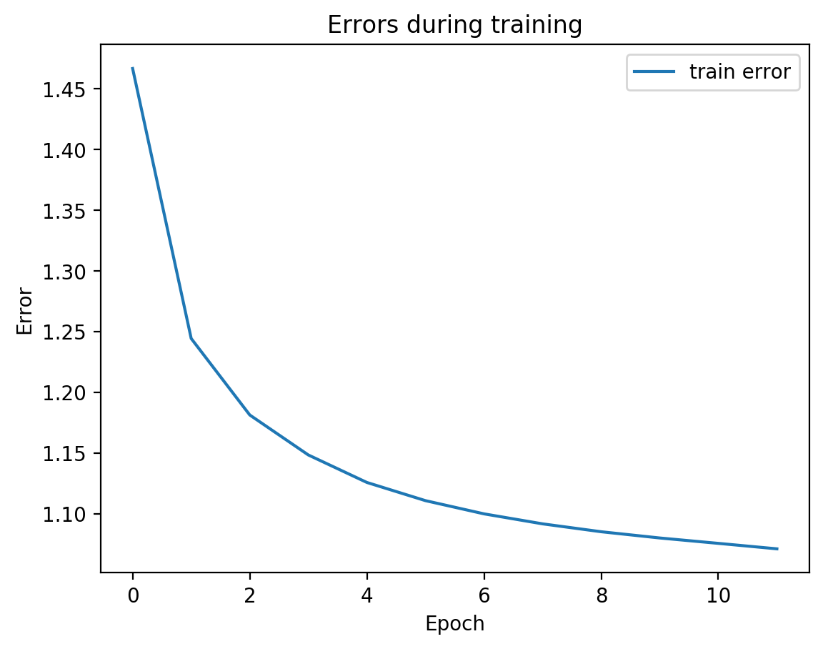
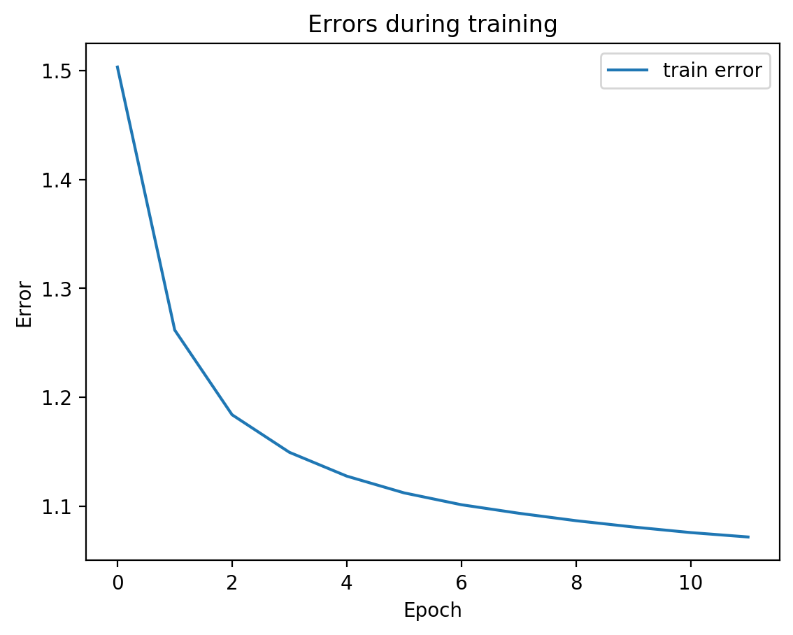
splitae = SplitAE(hidden_size=1024, num_hidden_layers=2, embed_size=10, training_epochs=10, batch_size=128,
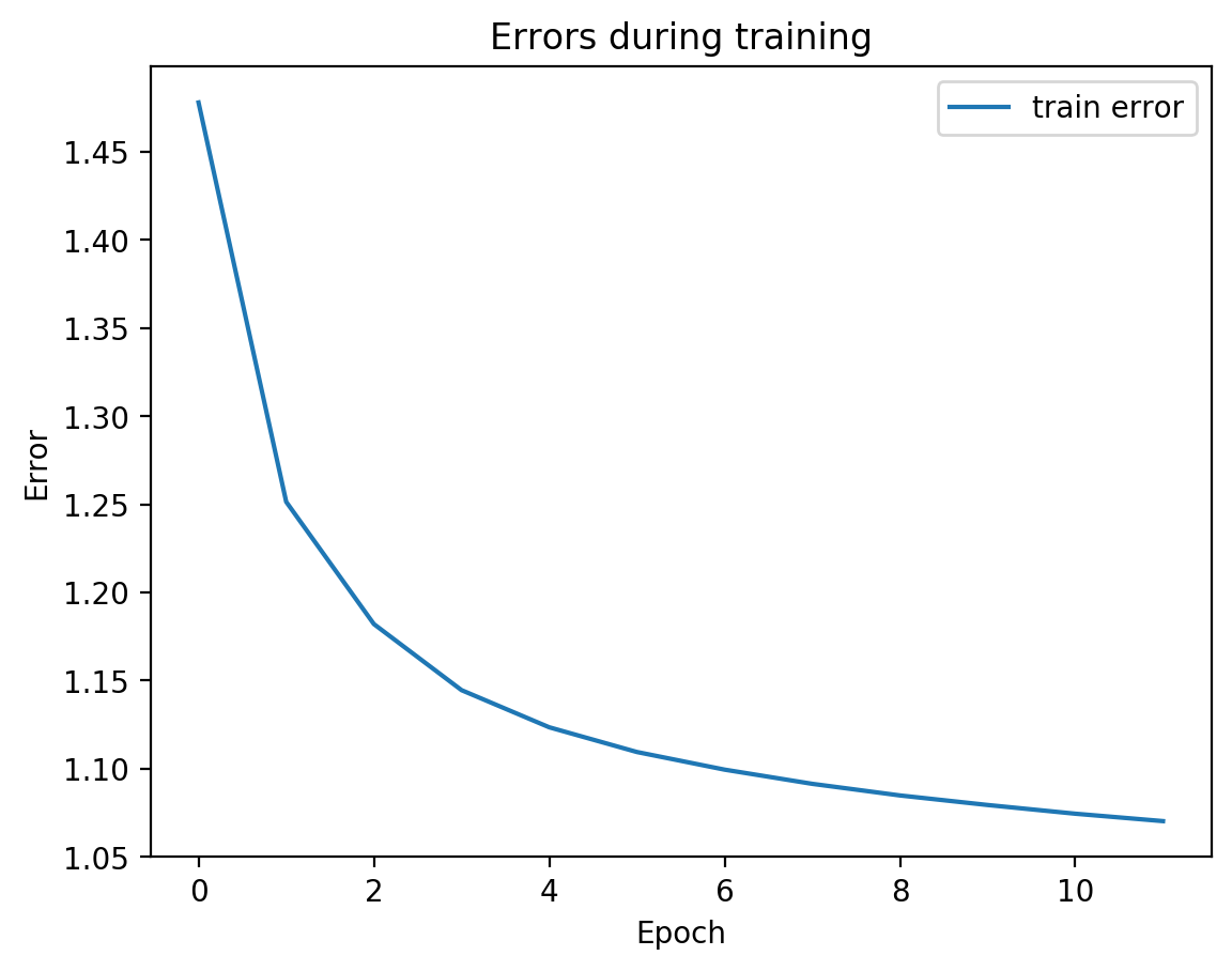
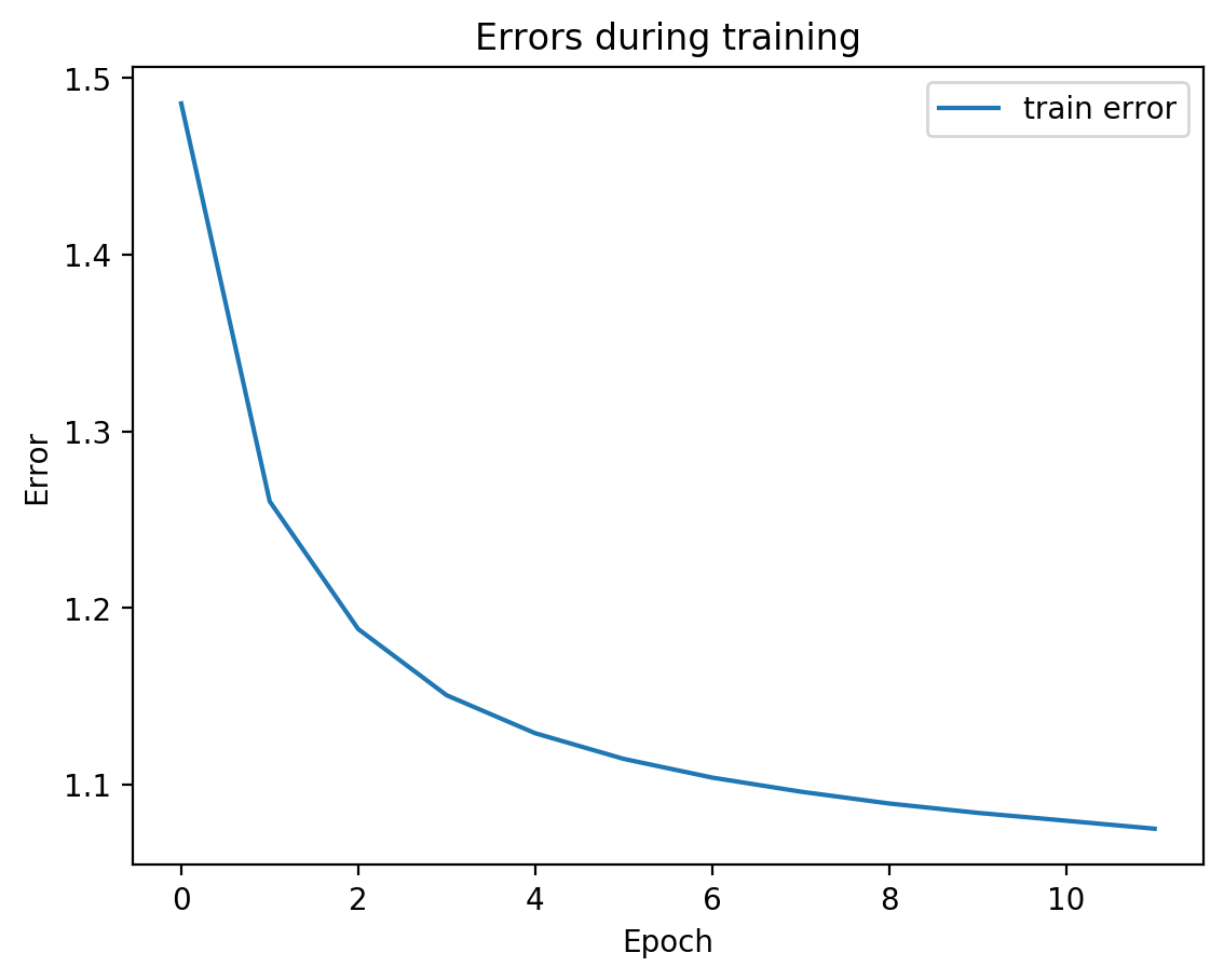
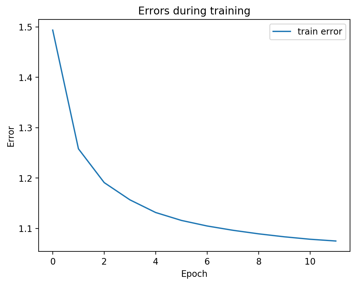
                  learning_rate=0.001, print_info=False, print_graph=True)
splitae.fit([view1, view2], validation_Xs=[testView1, testView2])
# if the named parameter validationXs is passed with held-out data, then .fit will print validation error as well.

Parameter counts:
view1Encoder: 1,863,690
view1Decoder: 1,864,464
view2Decoder: 1,864,464

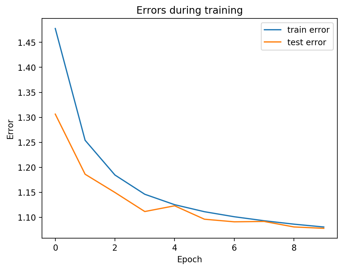
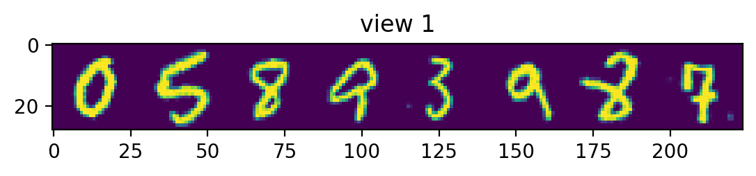
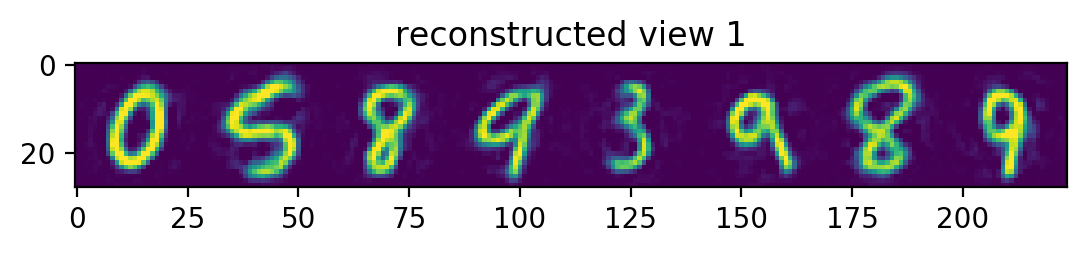
We can see from the graph that test error did not diverge from train error, which means we’re not overfitting, which is good! Let’s see the actual view1 recreation and the view2 prediction on test data:

MNIST_MEAN, MNIST_STD = (0.1307, 0.3081)
testEmbed, testView1Reconstruction, testView2Prediction = splitae.transform([testView1, testView2])
numImages = 8
randIndices = np.random.choice(range(len(testDataset)), numImages, replace=False)
def plotRow(title, view):
    samples = view[randIndices].reshape(-1, 28, 28)
    row = np.concatenate([*samples], axis=1)
    row = np.clip(row * MNIST_STD + MNIST_MEAN, 0, 1) #denormalize
    plt.imshow(row)
    plt.title(title)
    plt.show()
plotRow("view 1", testView1)
plotRow("reconstructed view 1", testView1Reconstruction)
plotRow("predicted view 2", testView2Prediction)

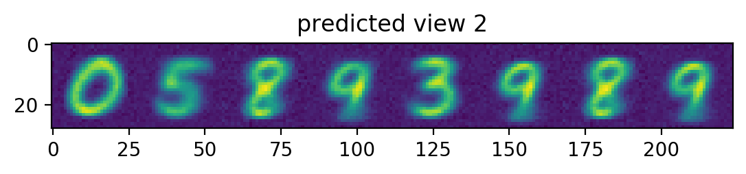
Notice the view 2 predictions. Had our view2 images been randomly rotated, the predictions would have a hazy circle, since the best guess would be the mean of all the rotated digits. Since we don’t rotate our view2 images, we instead get something that’s only a bit hazy around the edges – corresonding to the mean of all the non-rotated digits.

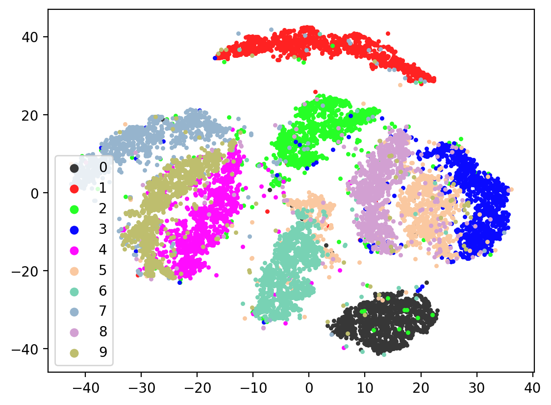
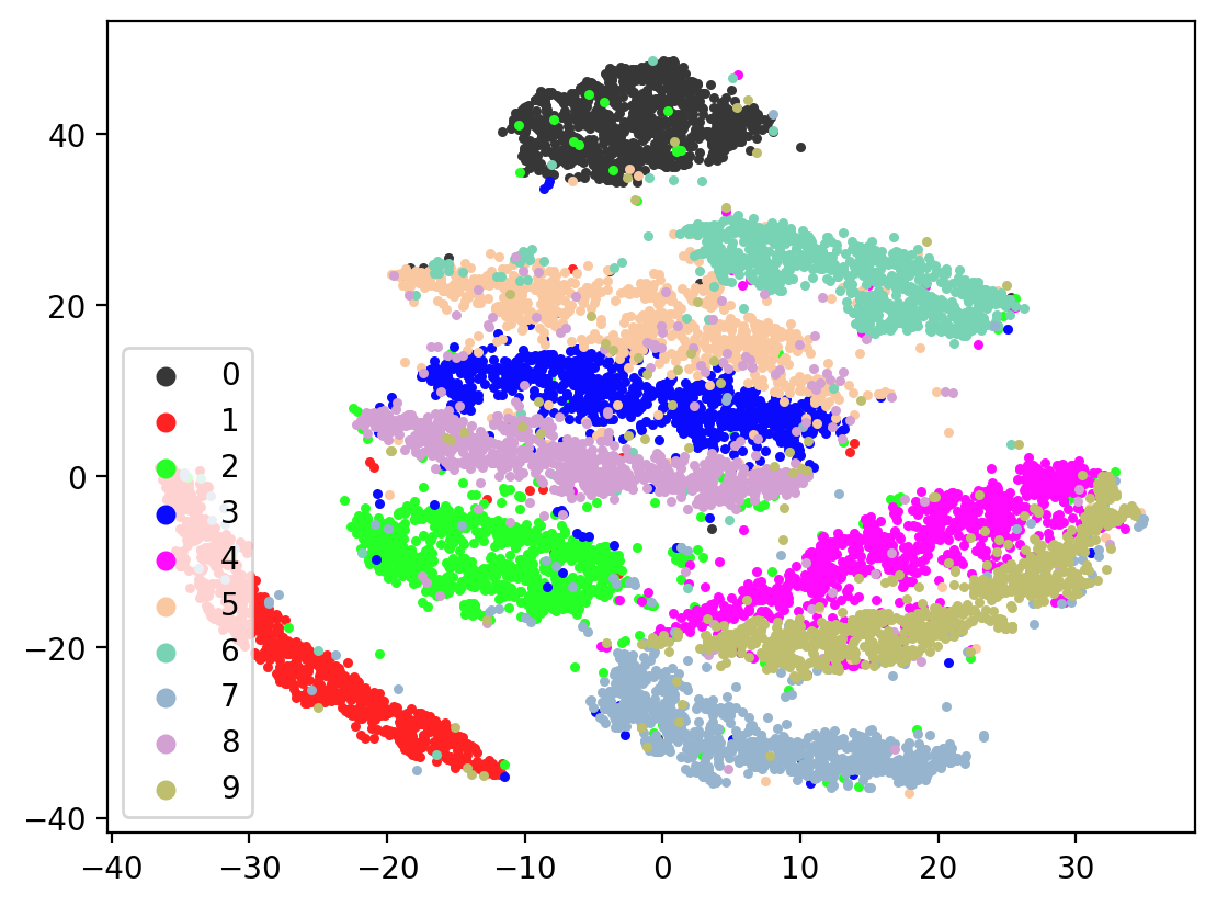
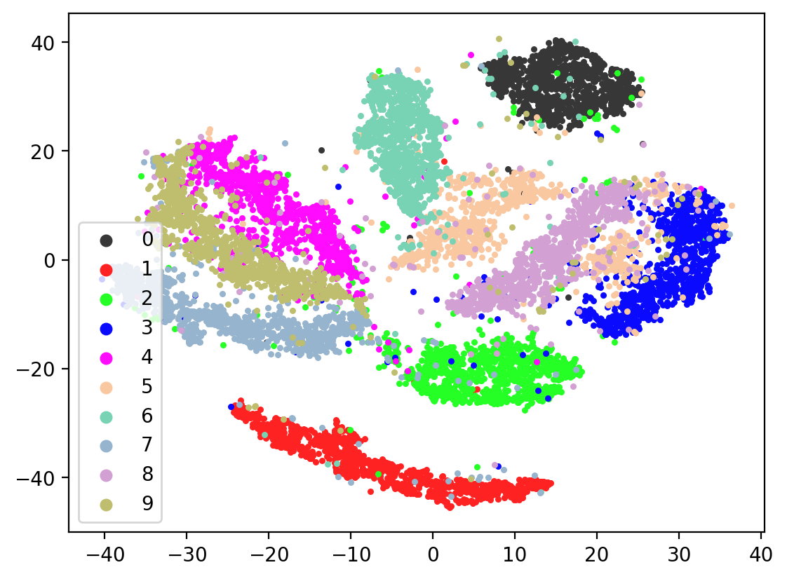
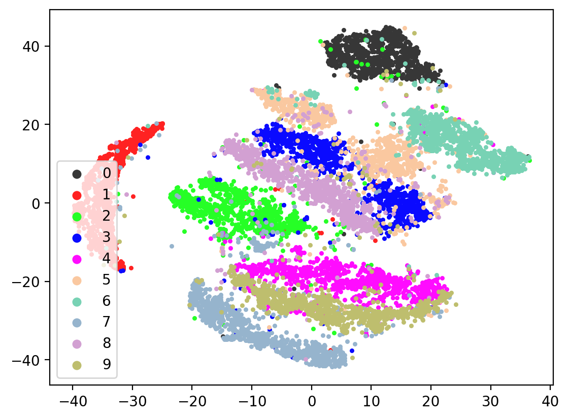
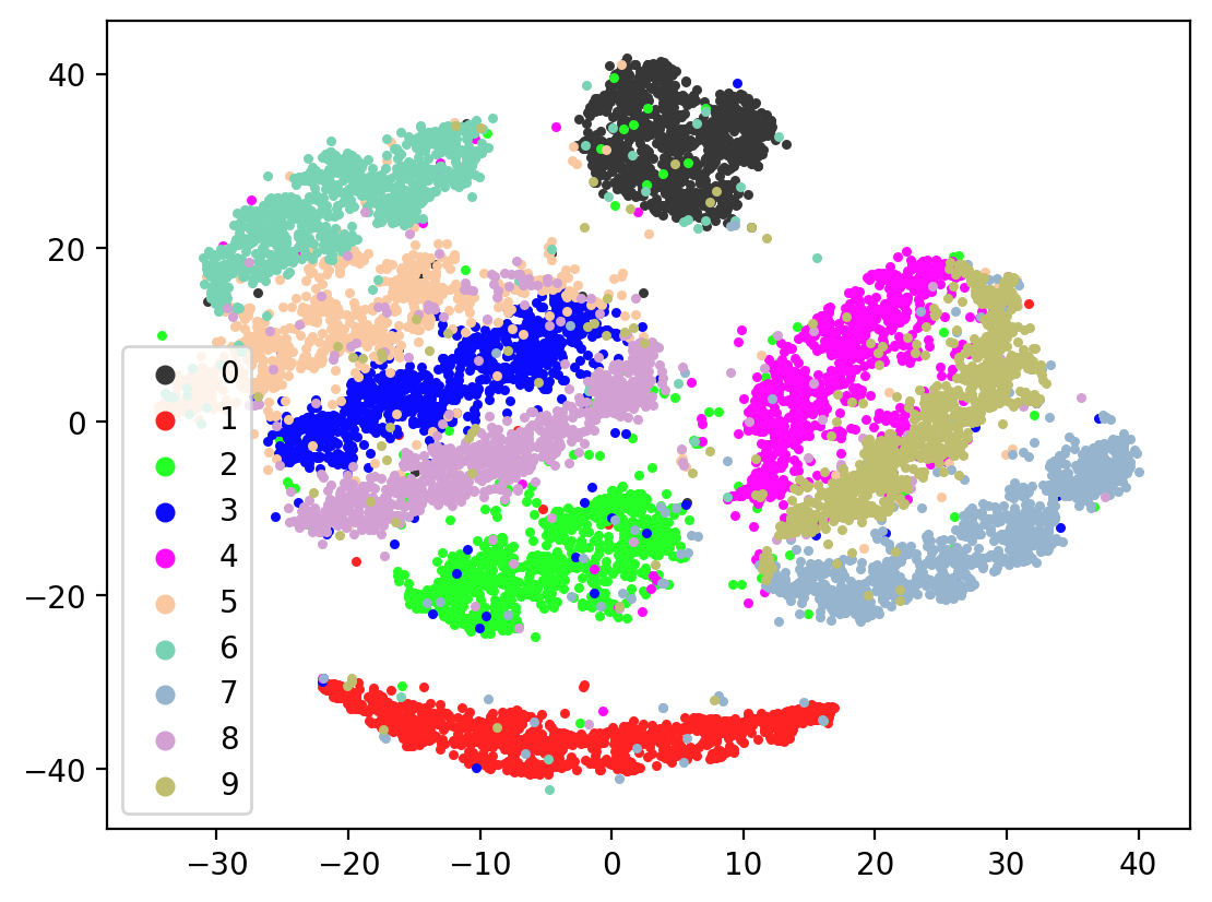
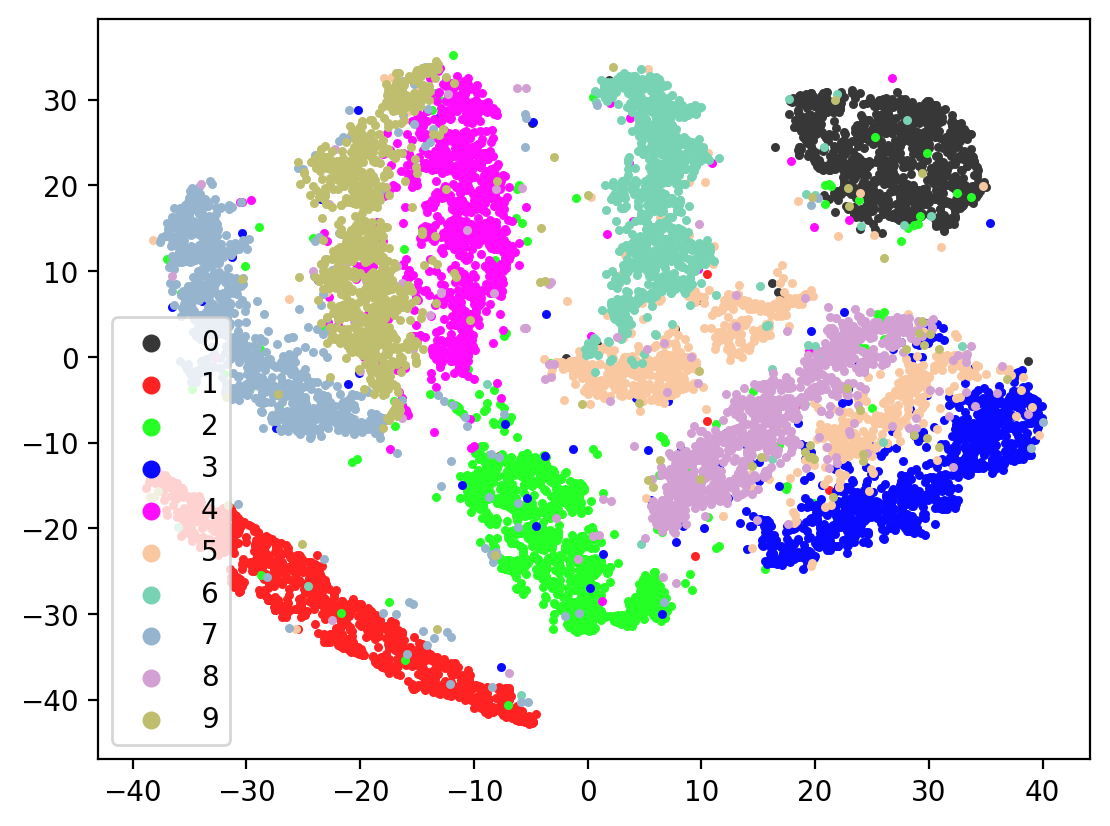
Next let’s visualize our 20d test embeddings with T-SNE and see if they represent our original underlying representation – the digits from 0-9 – of which we made two views of. In the perfect scenario, each of the 10,000 vectors of our test embedding would be one of ten vectors, representing the digits from 0-9. (Our network wouldn’t do this, as it tries to reconstruct each unique view1 image exactly). In lieu of this we can hope for embedding vectors corresponding to the same digits to be closer together.

%config InlineBackend.figure_format = 'retina'

tsne = TSNE()
tsneEmbeddings = tsne.fit_transform(testEmbed)

def plot2DEmbeddings(embeddings, labels):
    pointColors = []
    origColors = [[55, 55, 55], [255, 34, 34], [38, 255, 38], [10, 10, 255], [255, 12, 255], [250, 200, 160], [120, 210, 180], [150, 180, 205], [210, 160, 210], [190, 190, 110]]
    origColors = (np.array(origColors)) / 255
    for l in labels.cpu().numpy():
        pointColors.append(tuple(origColors[l].tolist()))

    fig, ax = plt.subplots()
    #scatter = ax.scatter(*tsneEmbeddings.transpose(), c=pointColors, s=5)
    for i, label in enumerate(np.unique(labels)):
        idxs = np.where(testLabels == label)
        ax.scatter(embeddings[idxs][:, 0], embeddings[idxs][:, 1], c=[origColors[i]], label=i, s=5)

    legend = plt.legend(loc="lower left")
    for handle in legend.legendHandles:
        handle.set_sizes([30.0])
    plt.show()

plot2DEmbeddings(tsneEmbeddings, testLabels)

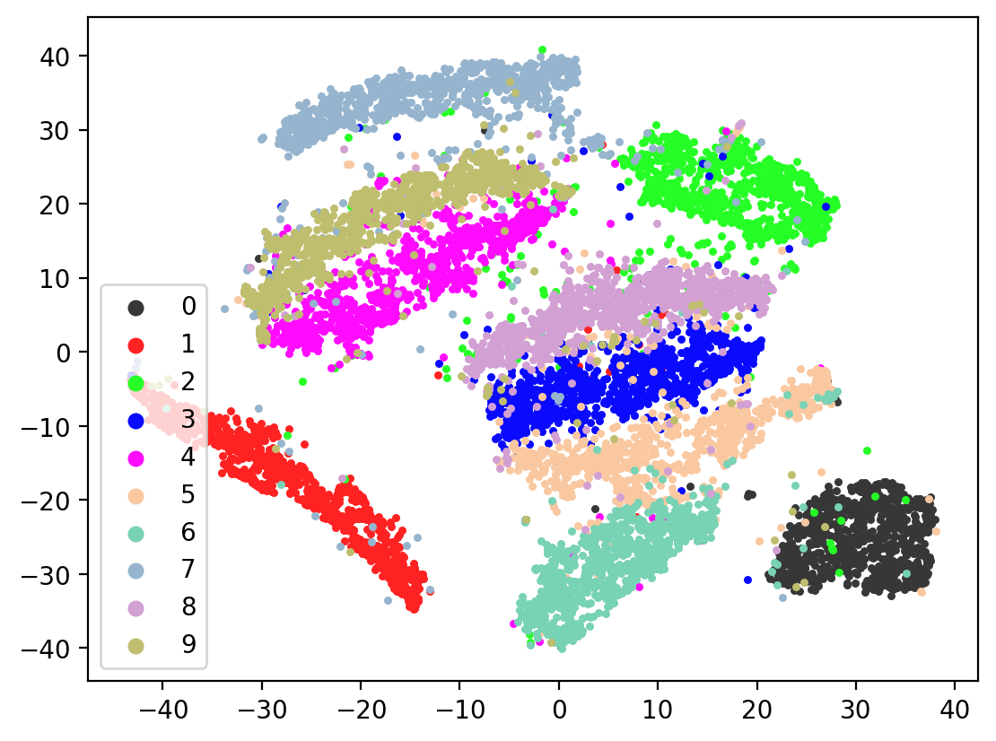
This is the image we’re trying to reproduce:

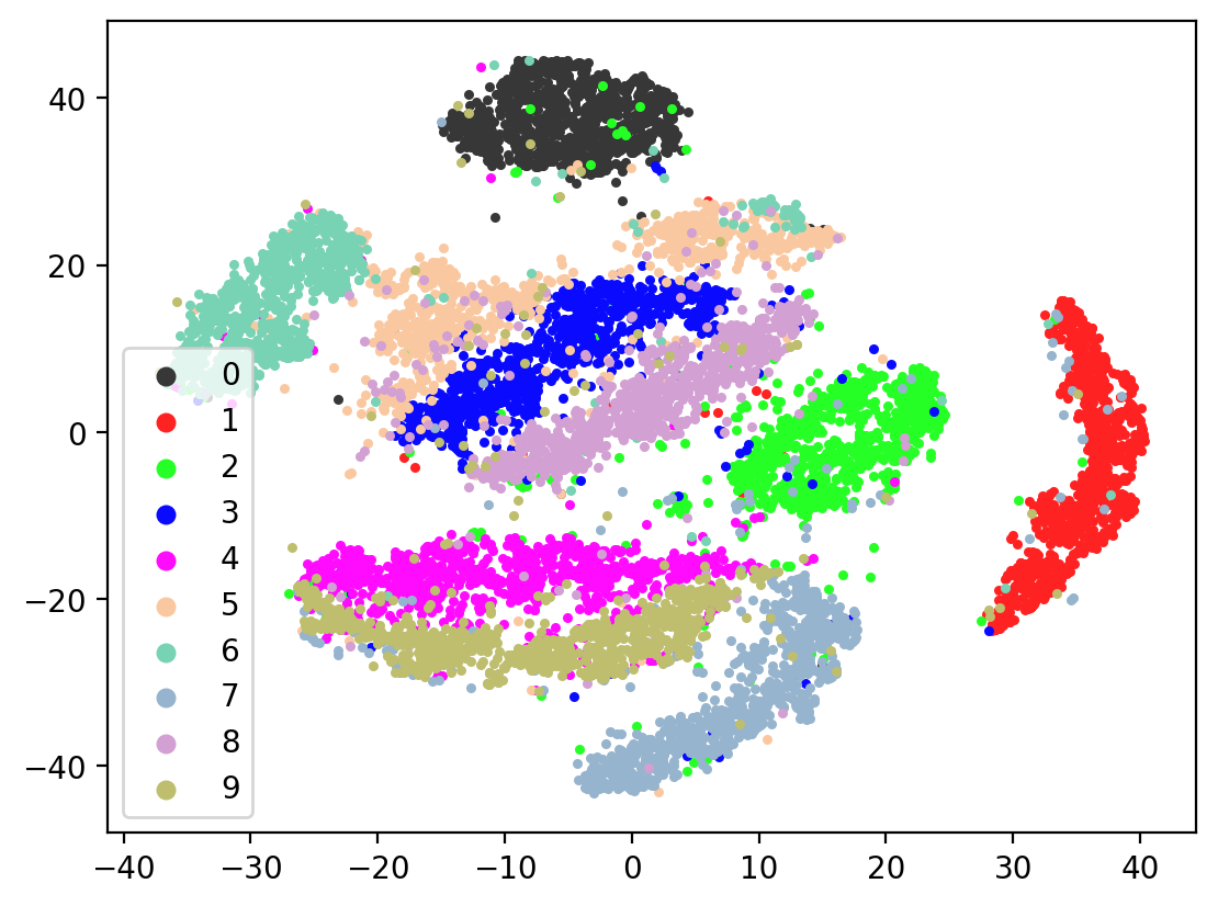
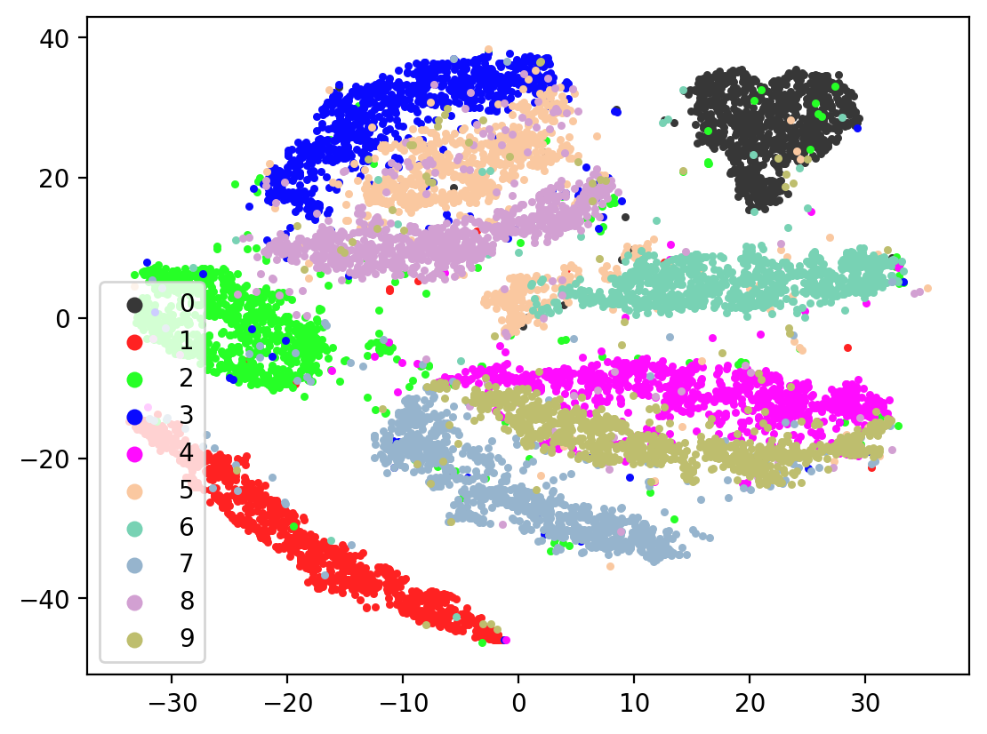
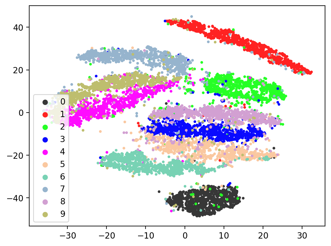
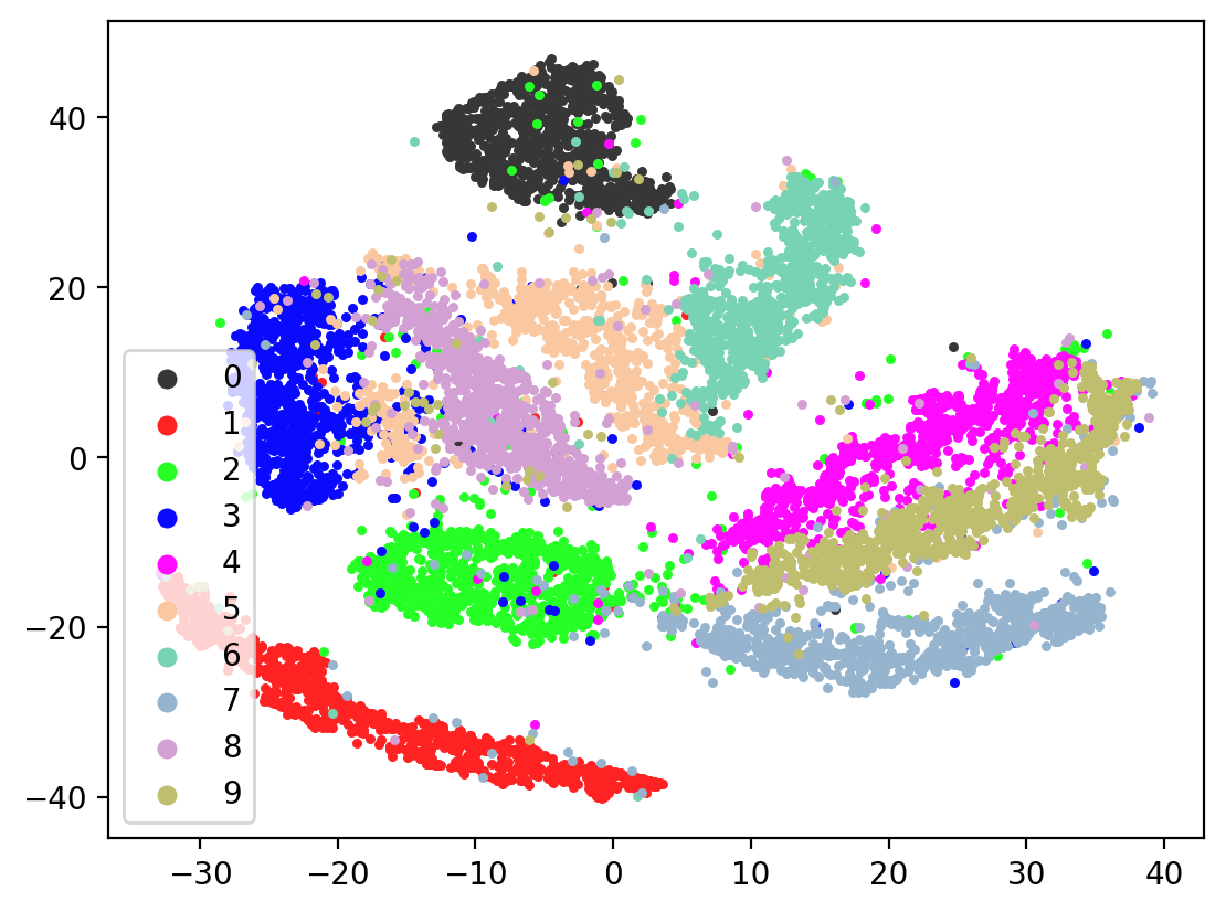
Lets check the variability of multiple TSNE runs:

for i in range(10):
    tsneEmbeddings = tsne.fit_transform(testEmbed)
    plot2DEmbeddings(tsneEmbeddings, testLabels)

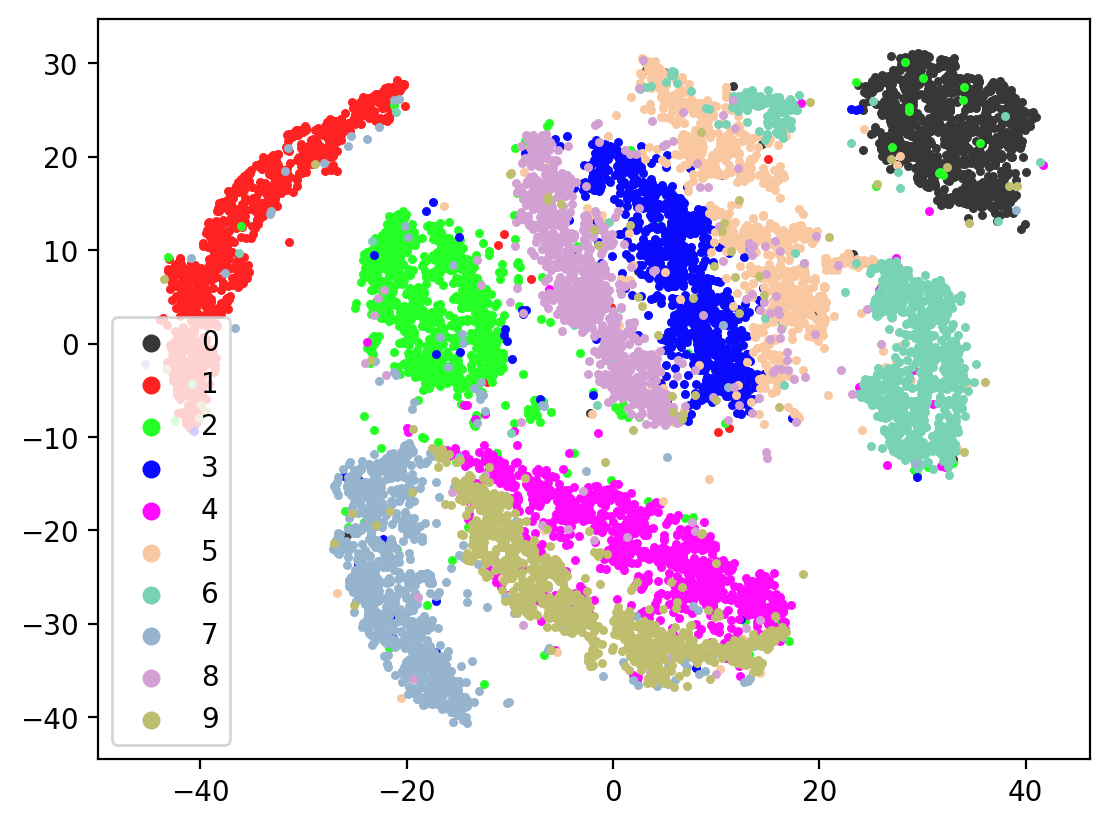
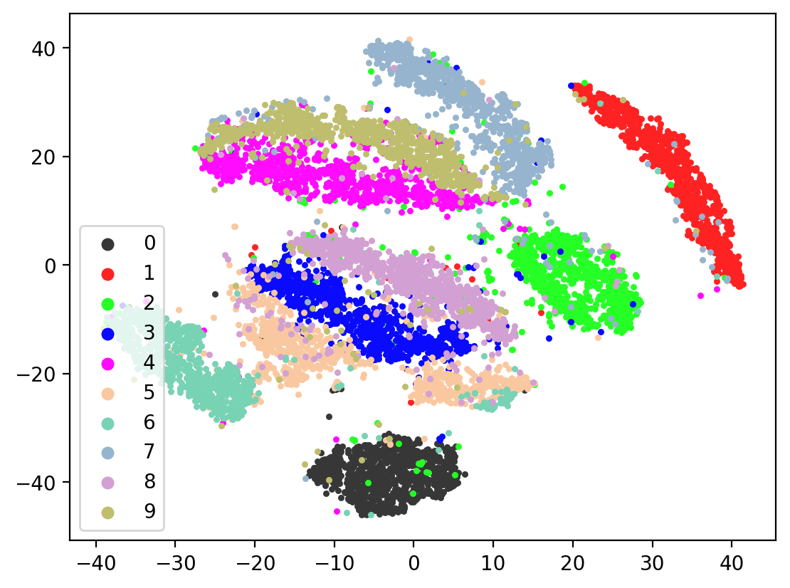
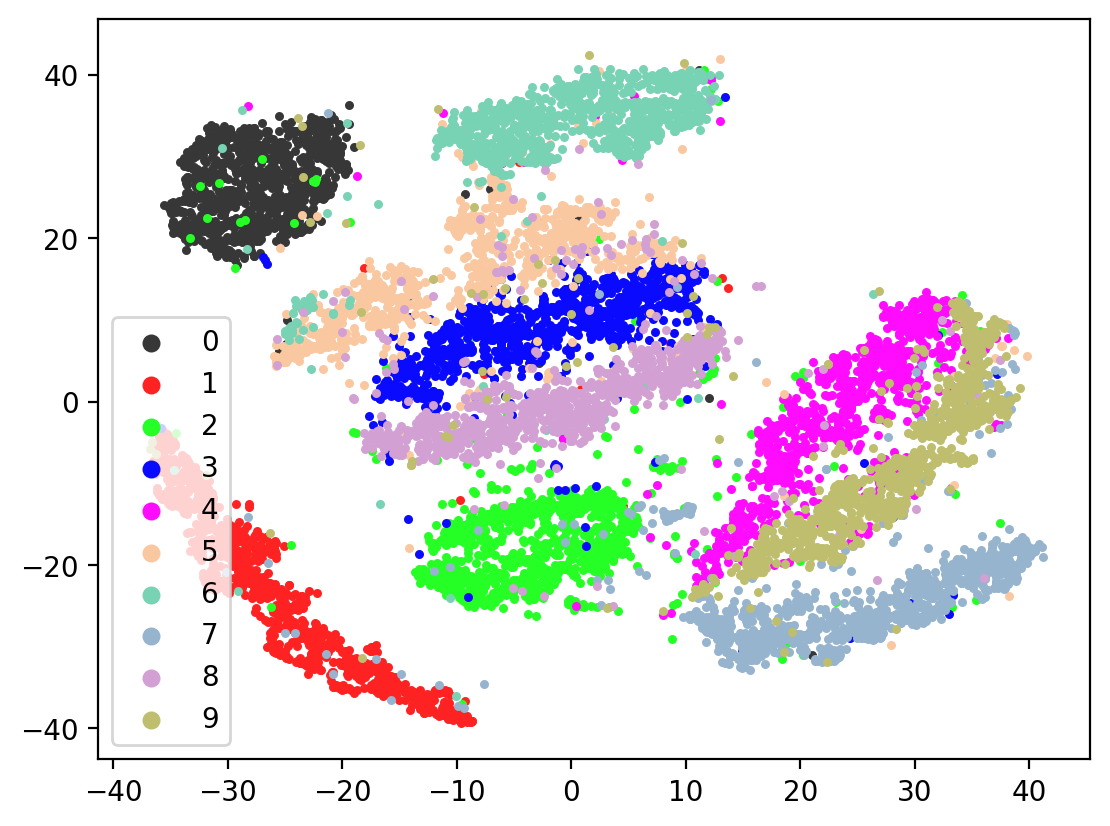
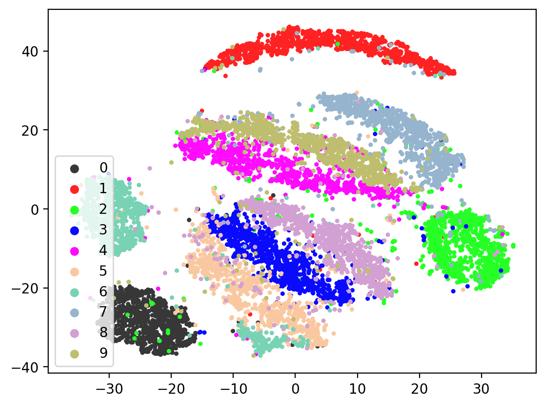
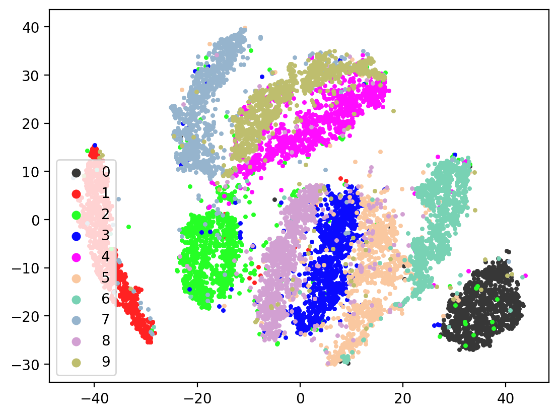
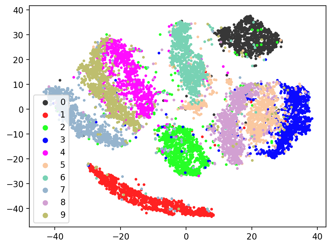
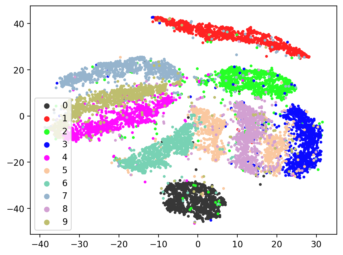
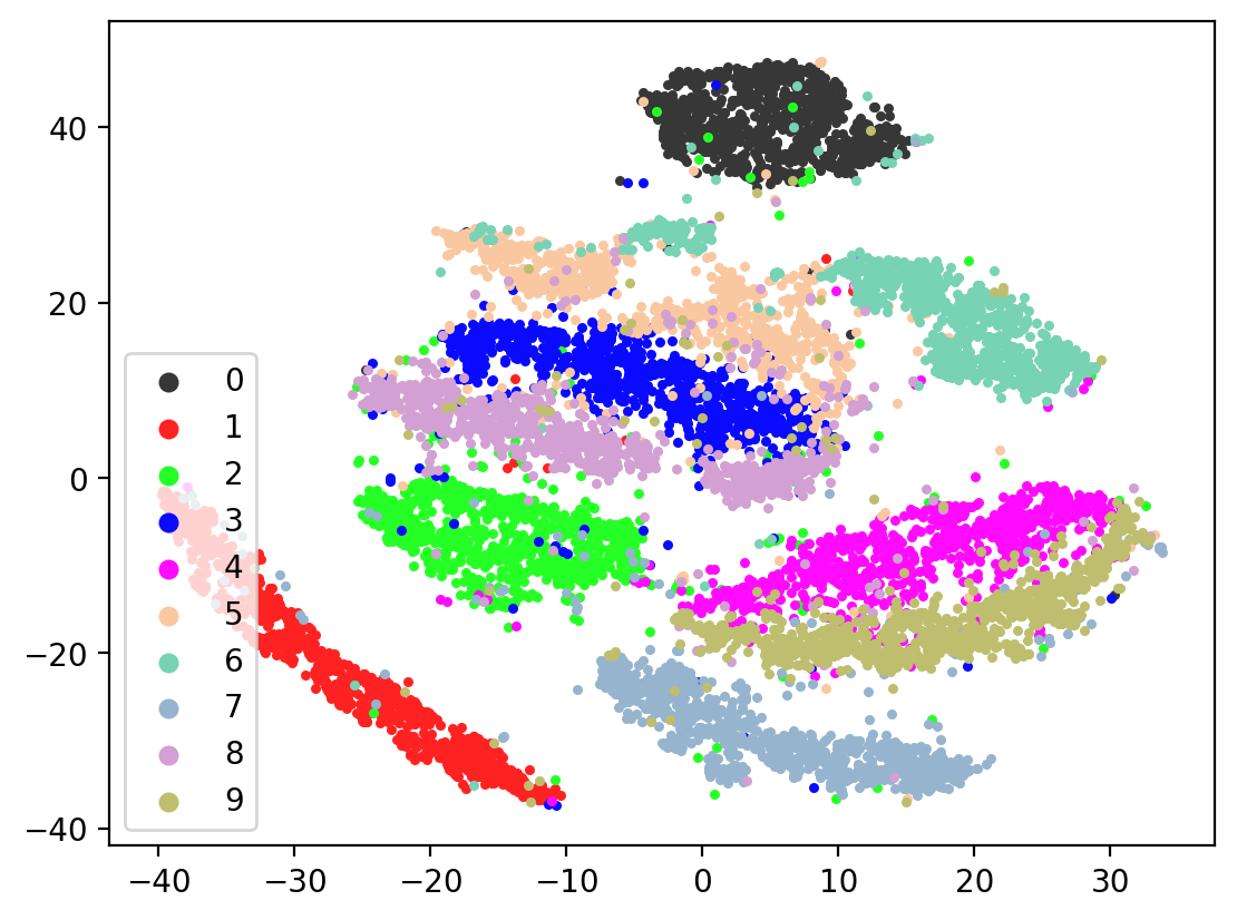
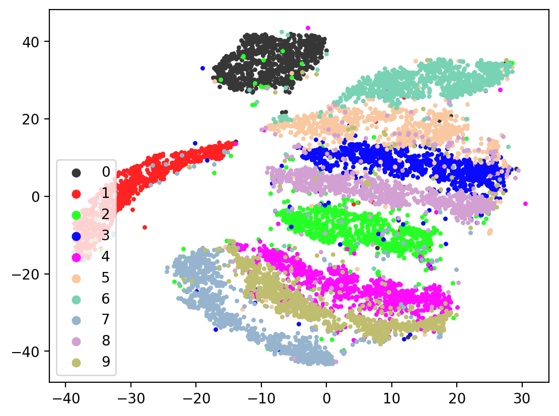
Now let’s check the variability of both training the model plus TSNE-ing the test embeddings.

for i in range(10):

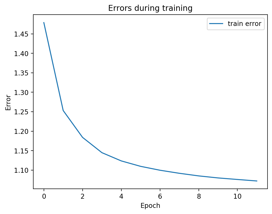
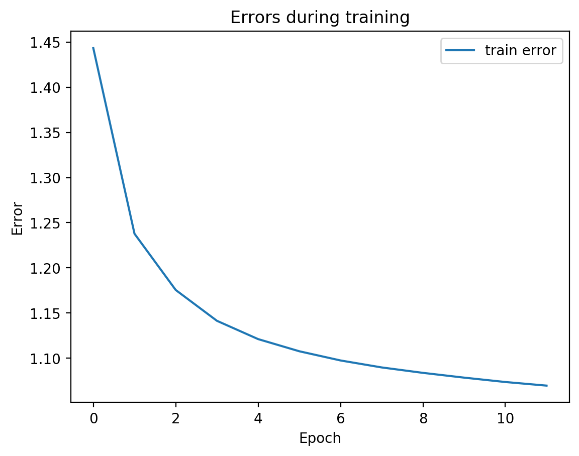
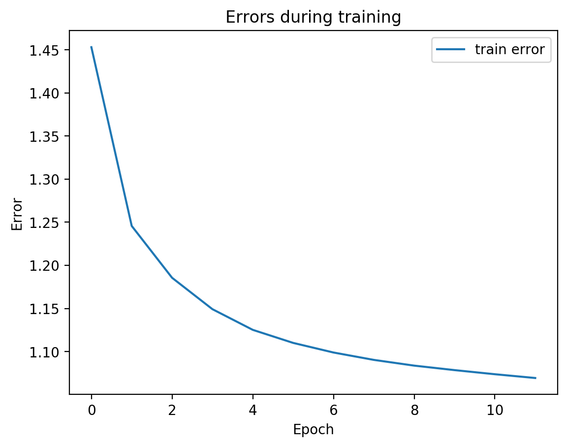
    splitae = SplitAE(hidden_size=1024, num_hidden_layers=2, embed_size=10, training_epochs=12, batch_size=128,
                      learning_rate=0.001, print_info=False, print_graph=True)
    splitae.fit([view1, view2])

    testEmbed, testView1Reconstruction, testView2Reconstruction = splitae.transform([testView1, testView2])

    tsneEmbeddings = tsne.fit_transform(testEmbed)
    plot2DEmbeddings(tsneEmbeddings, testLabels)

Parameter counts:
view1Encoder: 1,863,690
view1Decoder: 1,864,464
view2Decoder: 1,864,464

Parameter counts:
view1Encoder: 1,863,690
view1Decoder: 1,864,464
view2Decoder: 1,864,464

Parameter counts:
view1Encoder: 1,863,690
view1Decoder: 1,864,464
view2Decoder: 1,864,464

Parameter counts:
view1Encoder: 1,863,690
view1Decoder: 1,864,464
view2Decoder: 1,864,464

Parameter counts:
view1Encoder: 1,863,690
view1Decoder: 1,864,464
view2Decoder: 1,864,464

Parameter counts:
view1Encoder: 1,863,690
view1Decoder: 1,864,464
view2Decoder: 1,864,464

Parameter counts:
view1Encoder: 1,863,690
view1Decoder: 1,864,464
view2Decoder: 1,864,464

Parameter counts:
view1Encoder: 1,863,690
view1Decoder: 1,864,464
view2Decoder: 1,864,464

Parameter counts:
view1Encoder: 1,863,690
view1Decoder: 1,864,464
view2Decoder: 1,864,464

Parameter counts:
view1Encoder: 1,863,690
view1Decoder: 1,864,464
view2Decoder: 1,864,464

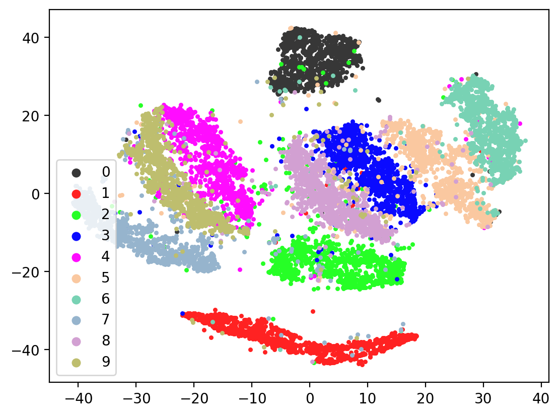
In most of the plots in the above cell we can see the distinct connected bands of the original figure, as well as the distinct black circular blob (corresponding to the digit 0, which appears easiest to learn). In some of the figures, a one or two bands are broken up. With more training of the network, though (stepping the learning rate), the bands converge less stretched (i.e. average distance between vectors of the same class is closer) blobs.